Numerical Simulation of Mechanical Systems

Prototype 1.0	Prototype 2.1

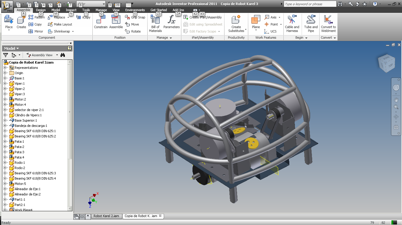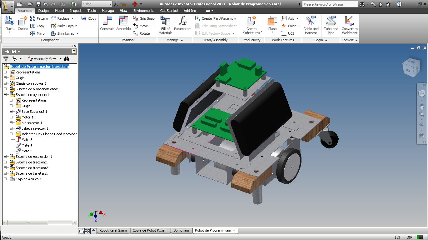In 2007, as an undergraduate mechanical engineering student, my friends and I were tasked with designing a two-wheeled robot that could follow a programmed path and pick up metallic coins along the way. It was an educational project, but even a simple goal like that demanded creativity, prototyping, and plenty of trial and error. The ideal outcome was a control scheme simple enough that a child could program the robot.

As with many university projects, time was short, manufacturing tools were limited, and the internet was far less useful than it is today—no GitHub, no Stack Overflow, and little access to papers beyond Wikipedia and the library. Most of our effort went into building the robot itself.

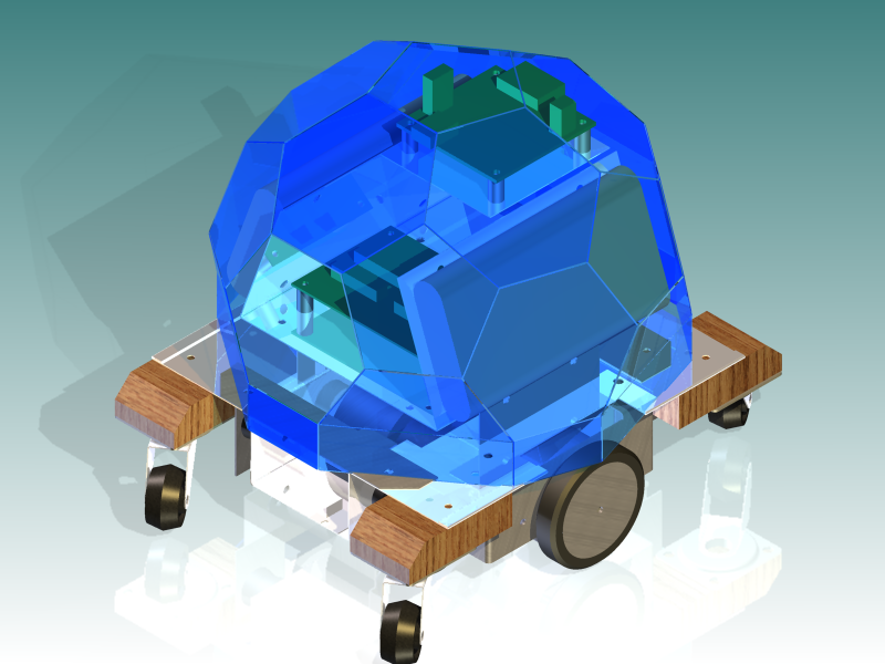
Once we had a minimal working prototype, the real challenge became clear: how do you make the robot follow a path with a little self-correction?

We tried several rudimentary control strategies, but none of them were general enough to be used in a real-world application.

Years later, I revisited this idea while teaching Python and ordinary differential equations. This time I choose to invests time in studying kinematic control approaches to describe the robot’s motion, while ODE solver were used to model classical damped systems such as vehicles. That gave me space to look again at the control problem and to see that there are two common philosophies for path following:

• Proportional–integral–derivative (PID) control reacts to the present error between a desired setpoint and the measured state. A familiar example is cruise control: when a car climbs a hill and slows down, the controller adjusts engine power to restore the target speed, with as little delay and overshoot as possible.
• Model predictive control (MPC) looks ahead: it predicts the robot’s future state and chooses control actions that keep it on the planned path.

Clearly, both approaches are valid and have their own advantages and disadvantages. But more importantly, they automatically adjust to the changing conditions of the environment. No need to program exceptions for each and every situation.

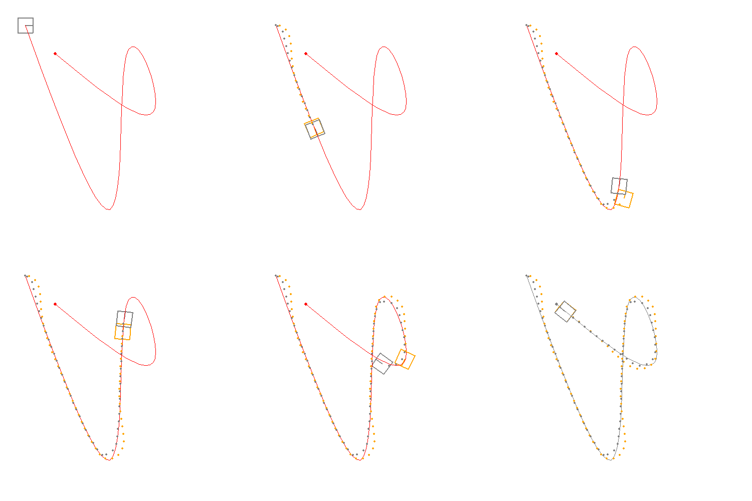
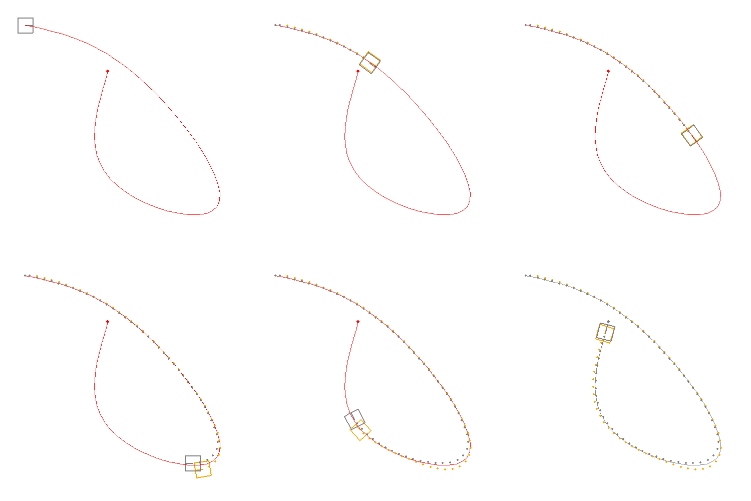
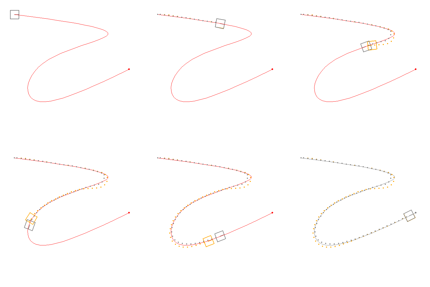
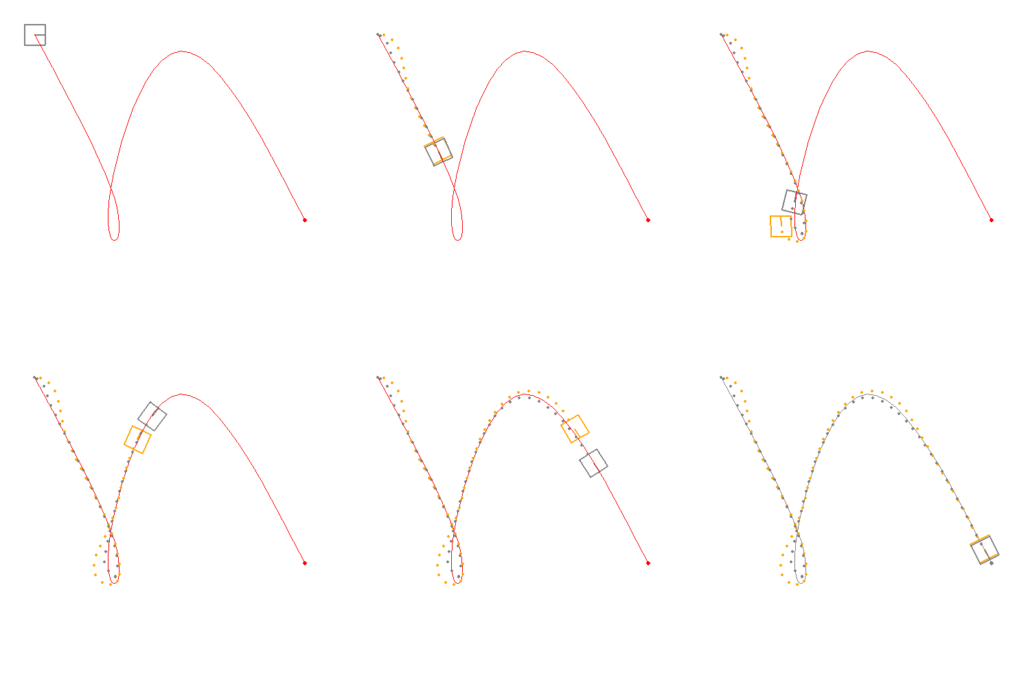
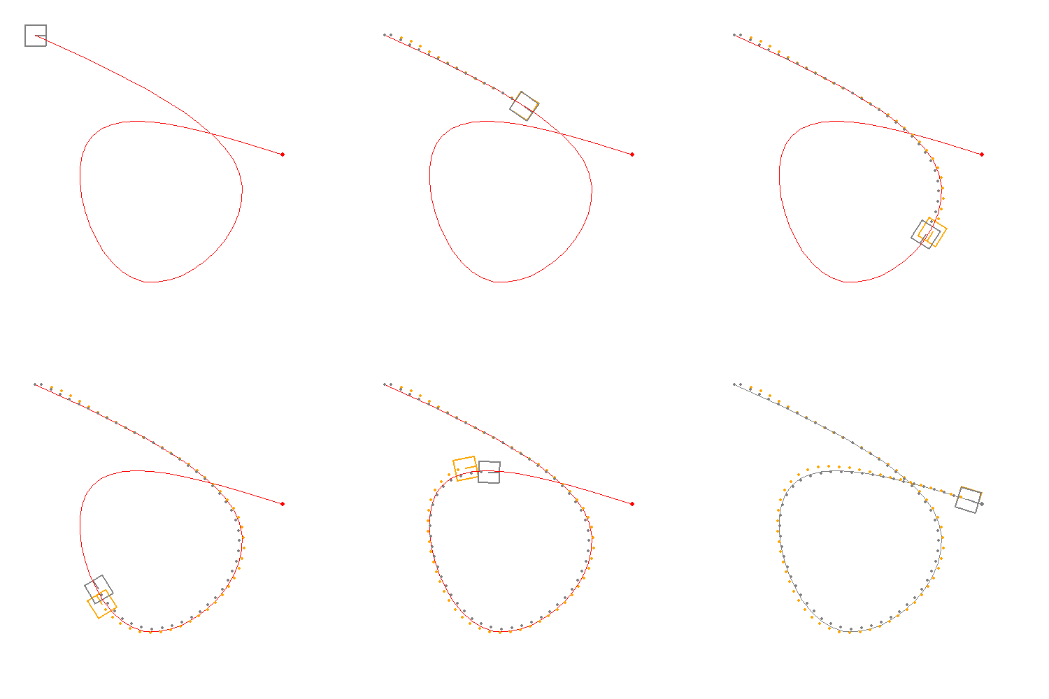
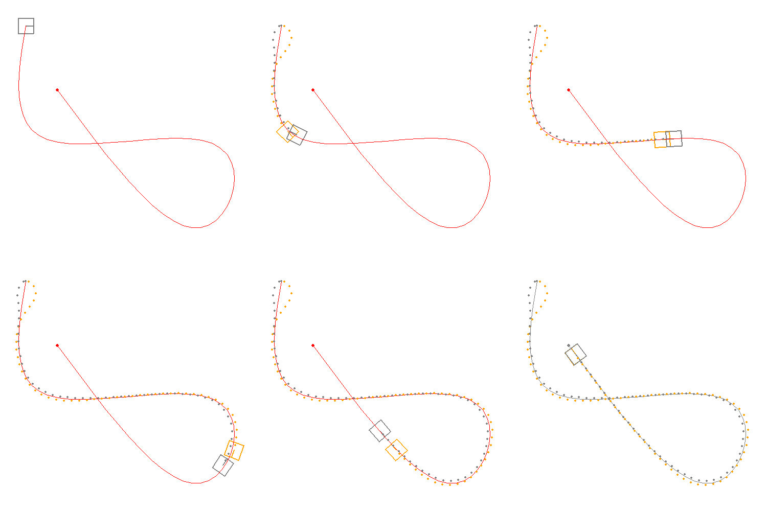
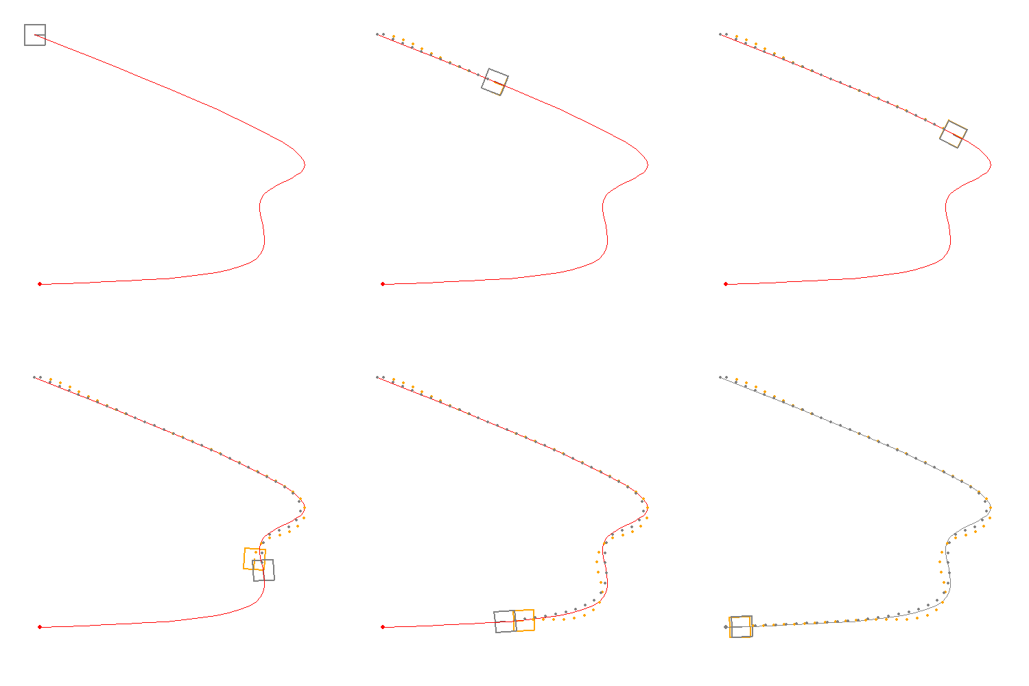
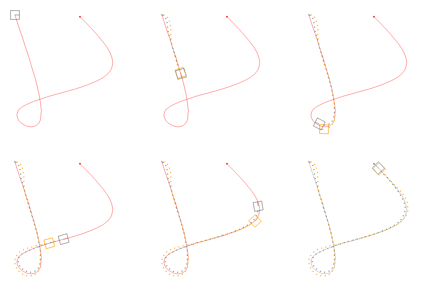
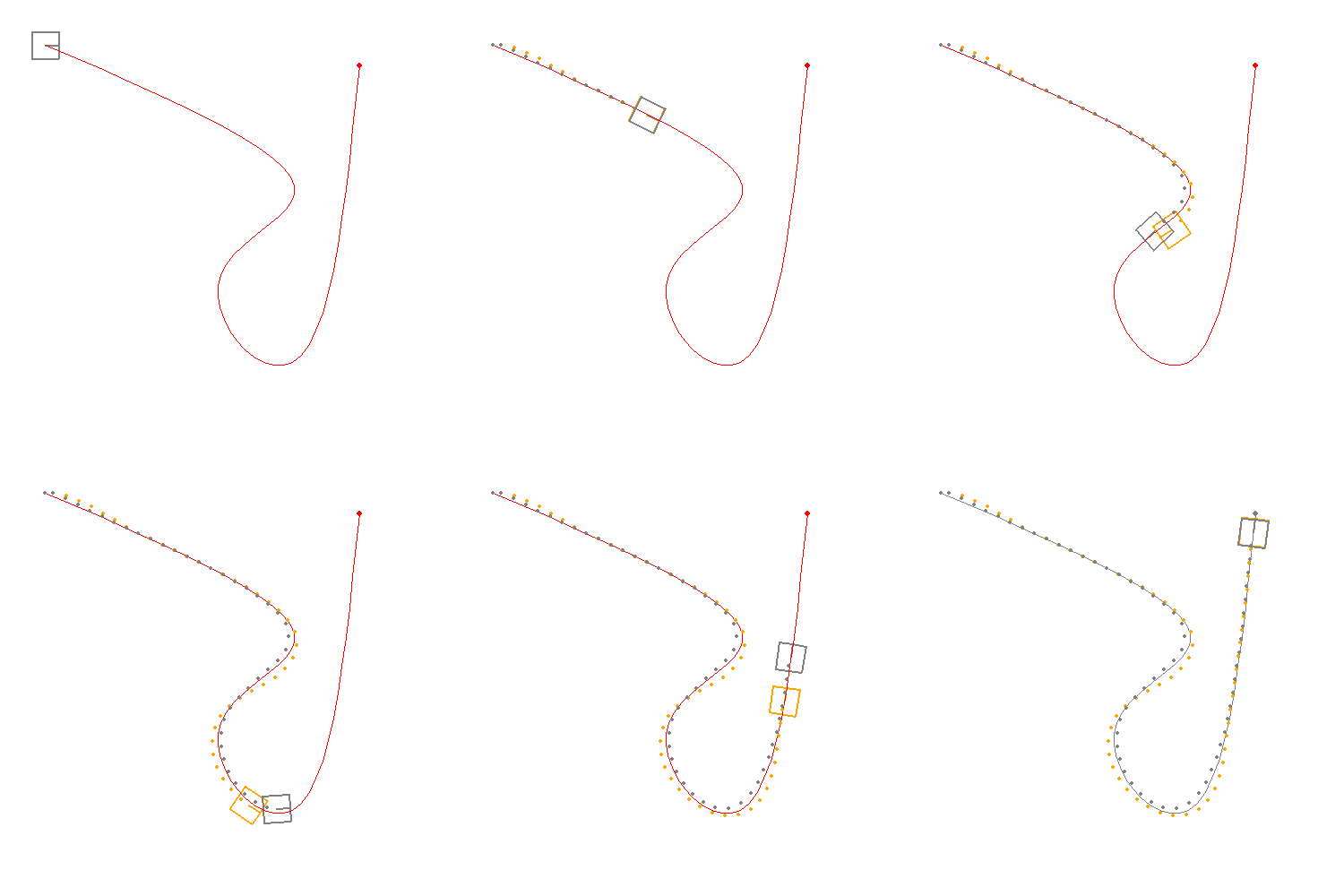
I implemented both strategies in Python and compared them on several test paths. To my surprise, MPC followed the paths much more closely than PID. It is a bit more complex to set up, but it proved to be the more robust approach.

Test Path	MPC (gray)	PID (orange)

In this project, I learned that the key to a successful control strategy is to understand the system dynamics and to be able to predict the future state of the system. And that the more complex the system, the more robust the control strategy. But I also become aware of two more popular control strategies:

• Pure pursuit control: aim at a look-ahead point on the path; simple, robust, very common on differential-drive robots and self-driving stacks, and
• LQR control: is a control strategy that seek to optimize a quadratic cost around a trajectory; lighter than full MPC, still “model-aware”.

I took inspiration on the work of KoKoLates to understand the dynamics of the robot and to implement the control strategies.